Cluster analysis
Get the stamped bricks' XRD dataset by Shawn Graham here and save it in a plain text file.
> xrd <- read.delim("bricks_xrd.txt", sep="\t")
> summary(xrd)
     Sample       Quartz           Augite        Haematite       Gehlenite        Calcite         Analcime    Muscovite
 se 14  : 2   Min.   : 11.00   Min.   : 10.0   Min.   : 3.00   Min.   : 2.00   Min.   :  2.0   Min.   : 5   Min.   : 3.00
 fal 1  : 1   1st Qu.: 36.75   1st Qu.: 29.5   1st Qu.: 8.00   1st Qu.:11.00   1st Qu.: 40.0   1st Qu.:11   1st Qu.: 9.00
 fal 2  : 1   Median : 52.00   Median : 54.0   Median :11.00   Median :30.00   Median : 66.0   Median :15   Median :12.00
 fal 3  : 1   Mean   : 59.24   Mean   : 60.1   Mean   :12.98   Mean   :30.46   Mean   : 64.9   Mean   :17   Mean   :14.24
 fnv13  : 1   3rd Qu.: 86.00   3rd Qu.: 91.5   3rd Qu.:17.00   3rd Qu.:47.00   3rd Qu.: 95.5   3rd Qu.:20   3rd Qu.:17.00
 fnv14  : 1   Max.   :117.00   Max.   :120.0   Max.   :34.00   Max.   :90.00   Max.   :127.0   Max.   :50   Max.   :42.00
 (Other):89                    NA's   :  9.0   NA's   : 8.00   NA's   :37.00   NA's   : 33.0   NA's   :51   NA's   :34.00
    Dolomite      Anorthoclase       Sanidine         Albite
 Min.   : 3.00   Min.   : 20.00   Min.   :  5.0   Min.   :  3.0
 1st Qu.:17.00   1st Qu.: 42.00   1st Qu.: 30.0   1st Qu.: 50.0
 Median :23.50   Median : 66.00   Median : 50.0   Median : 65.5
 Mean   :24.43   Mean   : 65.33   Mean   : 49.5   Mean   : 65.2
 3rd Qu.:32.00   3rd Qu.: 90.00   3rd Qu.: 65.0   3rd Qu.: 86.5
 Max.   :48.00   Max.   :115.00   Max.   :114.0   Max.   :117.0
 NA's   :26.00   NA's   : 47.00   NA's   : 70.0   NA's   : 50.0
hclust
Before creating the actual cluster dendrogram, we have to calculate the
distance matrix from our data frame. For this task we use the dist()
function:
> dist_xrd <- dist(xrd[-1])
(Note that the first column (label) is left intentionally out with the
xrd[-1] syntax, i.e. all columns but the first)
We are ready to create the dendrogram. The syntax is quite plain, even though the console output is not very satisfying. The cluster object is saved to another variable because we are going to plot it.
> clust_xrd <- hclust(dist_xrd)
> clust_xrd

Call:
hclust(d = d_xrd)

Cluster method   : complete
Distance         : euclidean
Number of objects: 96
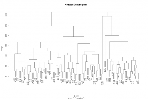
And now plot it:
> plot(clust_xrd)
Maybe adding the right label to each leaf:
> plot(clust_xrd, labels = xrd$Sample)
And here's the result:

Once you get acquainted with these functions, you can also get the plot with one single line:
> plot(hclust(dist(xrd[-1])), xrd$Sample, hang = -1, cex = 0.7)